Transformers from zero
This is a quick implementation of transformers that a friend of mine (link) and I made from zero with no guidance from the paper just to practice and understand better transformers. This is our explanation of transformers, therefore the notation and order of variables maybe change a bit.
The code can be found in the following link github.com/NotAnyMike/transformer
General
There are mainly 3 parts to this. Transformer start with the self-attention mechanism, scaling it into multiple heads we get the multi-head attention and finally by staking these together we get a transformer. The sections here are organized in those 3 steps.
1. Attention architecture
Let’s assume we have an input of \(n\) elements of length \(l\)
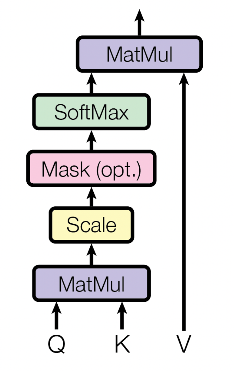
\[Q = V = K = \{q_{i,j}\} \in \mathbb R^{n \times l}\] \[Q V^T = S \in \mathbb R^{n \times n}\]\(S = \{s_{i,j}\}\) is basically the similarity matrix of the elements (how similar element \(i\) is to element \(j\)). The more similar the higher their multiplication will be and vice-versa.
Basically element \(j\) means \(e_j = \{v_{i,j}\}\) with \(i\in [1,2,3,...,n]\)
Therefore it is the same as
\[s_{a,b} = e_a \odot e_b = |e_a||e_b|\cos \theta\]It is just a way of measuring how alike two vectors are.
We make it a probability with softmax applied to each row or column depending on the order of multiplication we will follow, for simplicity, we will apply it over the row.
\[\text{softmax}( S)\]And self-attention basically is the result of weighting the original values of \(V\) with the result of the softmax
\[\text{softmax}( S)^T V\]One extra small thing we could do to improve training and convergence is to avoid the gradient tending to zero (similar to a vanishing gradient problem), remember that softmax flattens the bigger the absolute value gets. One way to avoid this is constraining \(S\) to grow significantly. We could control the variance of the model.
Let’s assume \(\text{var} (q_{i,j}) = \sigma^2\), because part of the matrix multiplication operation to calculate \(S\) includes summing over the \(l\) product of elements, the variance will be \(l\) times \(\sigma^2\). To avoid the product potentially having bigger and bigger values we could scale \(S\) down by \(\sqrt l\) so the variance gets scaled down by the same amount it increased due to the matrix multiplication. Therefore the scaled attention equation becomes
\[\text{softmax}\left(\frac{ S}{\sqrt l} \right)^TV\]Masking the future out
Sometimes when working with a sequence of values, it is important to avoid passing information about the future (because during inference the model will not have future information or because we want to estimate the next value). Given that \(Q, V, K\) includes all the sequences (all of the \(n\) vectors).
For this reason, we can just multiply the element scaled similarity matrix by a mask. Let’s imagine we are in the \(j\)th element and want to predict the \(j+1\)th element, therefore the mask will be \([1,1,1,...,0,0,0]\) where all the elements after \(j\) will be zero. We are allowed to train not just in the \(j\)th element but in any element, therefore the mask masking each of the posterior (aka future inputs) will look like
\[M = \{m_{i,j}\} \in \mathbb R^{n\times n} = \left( \matrix{ 1 & 0 & 0 & 0 & ...\\ 1 & 1 & 0 & 0 & ...\\ 1 & 1 & 1 & 0 & ... \\ & \text{...} & & & 1 } \right)\]Including the mask into the attention equation we have
\[A = \text{softmax}\left(M\frac{ S}{\sqrt l} \right)^TV\]Therefore because \(A\) is just the same input but weighted differently we get that \(Q,V,K,A \in \mathbb R^{l\times n}\)
2. Multi-head attention architecture
There are three improvements we can apply to the current self-attention architecture.
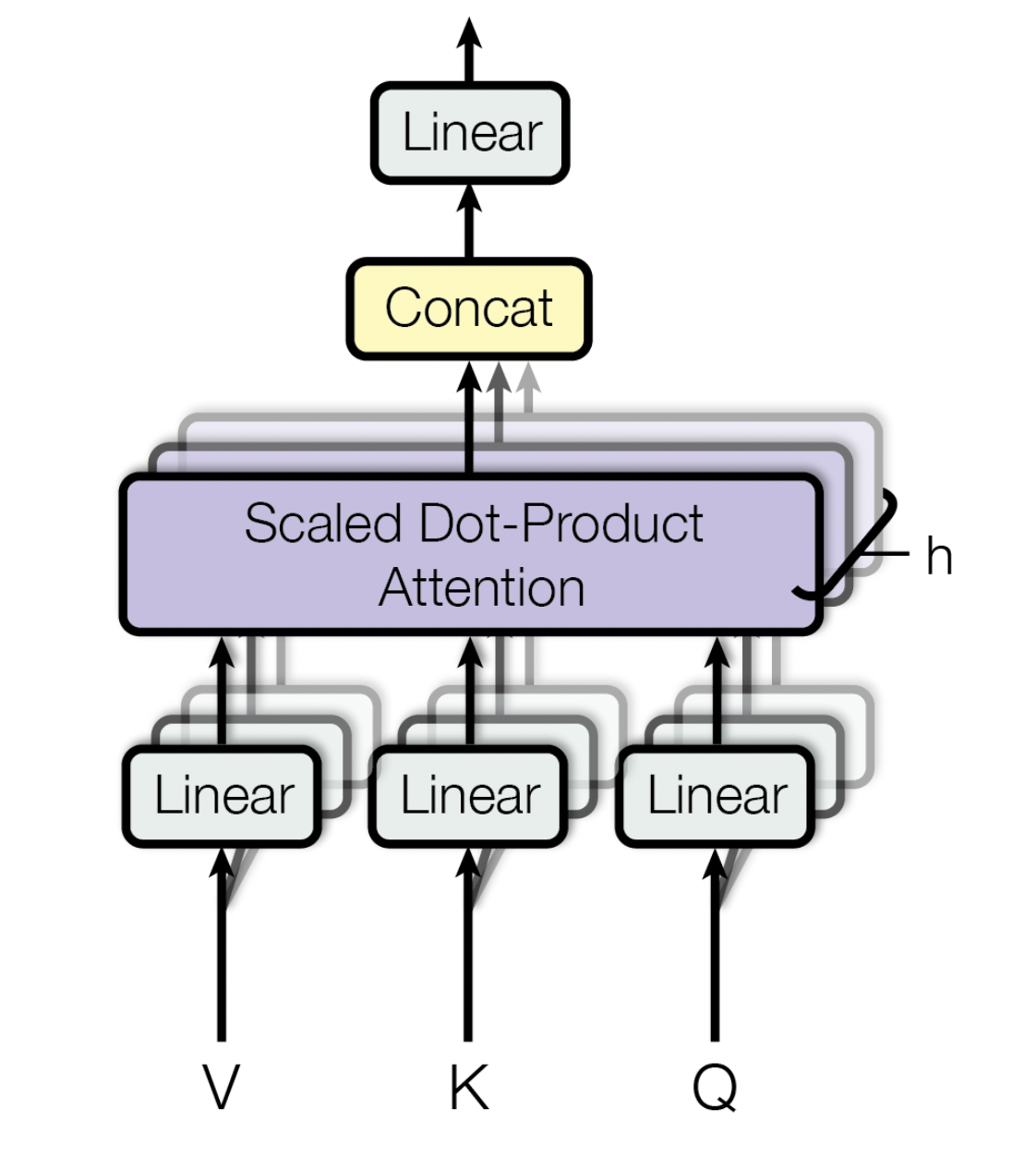
First, to allow the network to transform the network (that is why it is called a transformer), we could improve the architecture by adding one linear layer just before the similarity matrix operation.
\[Q = f_\theta(X)\\ K = f_\gamma(X)\\ V = f_\beta(X)\]Where \(\theta, \gamma, \beta\) are the parameters of each layer and \(X\) is the input vector. Now \(Q,K,V\) may not be equal.
A second improvement we could add is to stack in parallel several of these operations \(h\) times. the way doing it is by simply expanding the parameters \(\theta, \gamma\) and \(\beta\), \(h\) times and then reshaping to \(h \times ...\). Therefore
\[Q' = f_{\theta'}(X) \in \mathbb R^{h \times l \times n} \\ K' = f_{\gamma'}(X) \in \mathbb R^{h \times l \times n}\\ V' = f_{\beta'}(X) \in \mathbb R^{h \times l \times n} \\ \\ S = Q'^T V'\in \mathbb R^{h \times n \times n}\\ \\ A' = \text{softmax}\left(\frac{ S}{\sqrt l} \right)^TV' \in \mathbb R^{h\times l\times n}\]To keep the same output dimension as the original self-attention mechanism we can flatten \(A'\) and add a linear layer from \(h \times l \times n\) to \(l \times n\) so the final equation for the multi-head attention mechanism is
\[A = f_{\phi}(A_\text{flatten}) \quad \text{with} \quad A_\text{flatten} \in \mathbb R^{hln}\]So as result we get \(A \in \mathbb R^{l \times n}\) and we can add an extra dimension \(b\) for the batch size.
3. Transformer architecture
The last step to build a transformer is to stack together several multi-head self-attention mechanisms in a specific order \(N\) times.
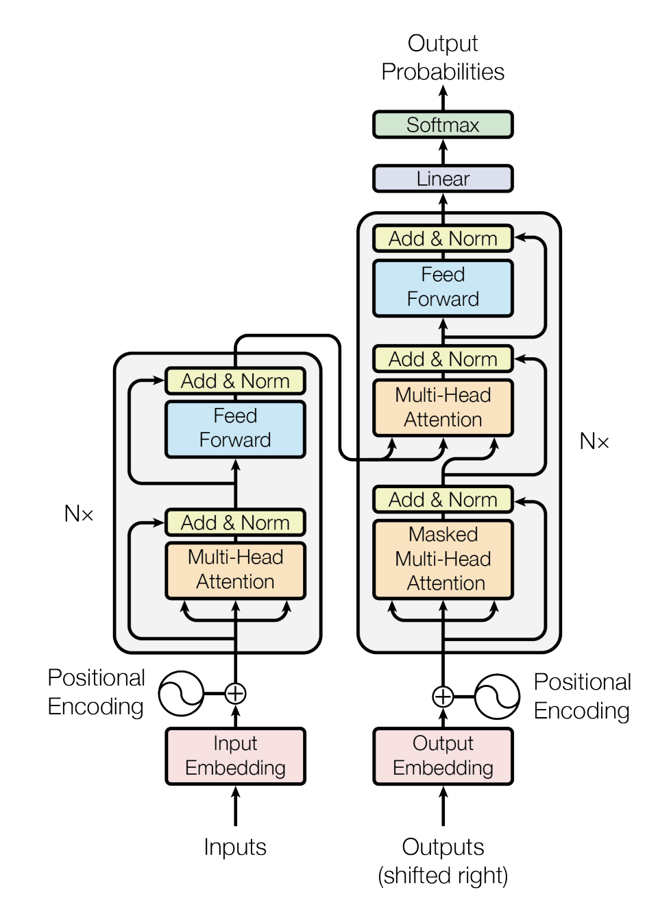
Positional encoding and input embeddings are an essential part of the architecture, but here we assume that \(X\) already contains both.
We will connect each of the outputs of the encoding transformers to the output of the next. For the decoder we will do the same, i.e. each output of the decoder is the input for the first masked multi-head attention’s input of the next decoder. Additionally, the output of the last encoder transformer is connected to all the input of the second multi-head attention of all \(N\) decoders.
To finish, we add a linear layer and softmax function to predict the probability of the next element of the sequence based on the vocabulary.